5 Describing and Visualizing Data

In this chapter we’ll work through a few examples of viewing, summarizing, and visualizing data. We’ll avoid importing files to make it as easy as possible to follow along.

Viewing Data

First, we’ll read in the powerlifting.csv file in the data folder.

data <- read.csv("power.csv")

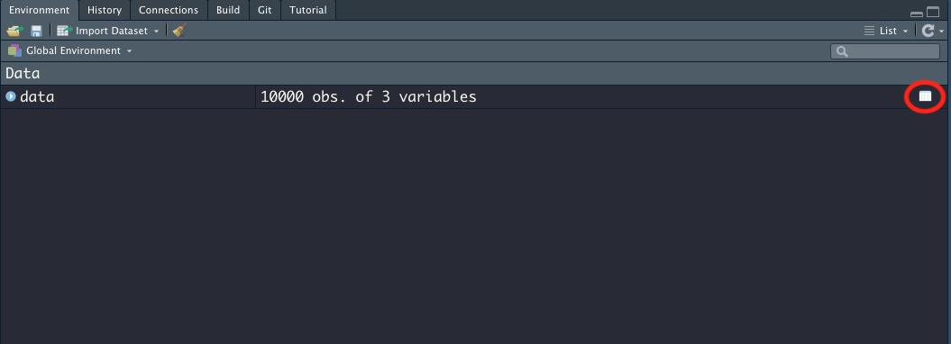
After running the code above, you should see an object called data under the Environment tab in the upper right pane of RStudio. If you click on the white grid icon, RStudio will display the data in tabular form.

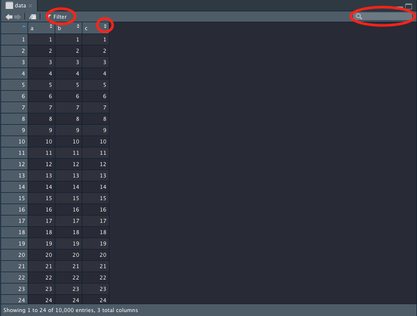
In this tabular view you can filter columns, arrange columns by ascending or descending values, and search values.

Another way to get the feel for an entire dataset is with the str() function. The benefit of the str() function is that the variable type is also displayed.

str(data)

'data.frame':   24 obs. of  6 variables:
 $ subject       : int  1 2 3 4 5 6 7 8 9 10 ...
 $ sex           : chr  "M" "M" "M" "M" ...
 $ self_ID       : chr  "endurance" "power" "power" "endurance" ...
 $ mass_kg       : num  65 80 71 64.5 73 ...
 $ VJ_power_watts: num  4203 5332 4431 3256 4001 ...
 $ WG_power_watts: int  809 995 856 595 707 956 870 966 1100 1188 ...

If you’re only interested in viewing the first few rows or last few rows of data you can use the head() and tail() functions, respectively:

head(data) # First 6 rows
tail(data) # Last 6 rows

  subject sex   self_ID  mass_kg VJ_power_watts WG_power_watts
1       1   M endurance 65.00000       4203.498            809
2       2   M     power 80.00000       5332.476            995
3       3   M     power 71.00000       4430.985            856
4       4   M endurance 64.50000       3256.266            595
5       5   M endurance 73.00000       4001.481            707
6       6   M     power 81.81818       5289.559            956
   subject sex   self_ID  mass_kg VJ_power_watts WG_power_watts
19      19   F     power 48.00000       3306.285            540
20      20   F     power 75.00000       3769.716            618
21      21   F     power 75.90909       3286.867            752
22      22   F endurance 55.90909       2572.519            622
23      23   F endurance 50.00000       2283.564            492
24      24   F     power 70.45455       4140.660            951

Sometimes it’s useful/convenient to access certain attributes of the data frame, such as the column names. A few of the functions for accessing attributes are provided below.

dim(data)        # Dimensions
nrow(data)       # Number of rows
ncol(data)       # Number of columns
colnames(data)   # Column names

Data Summaries

One of the quickest and most useful ways to produce a data summary is with the summary() function. This function is versatile and works well with both continuous and categorical data:

summary(data)

    subject          sex              self_ID             mass_kg     
 Min.   : 1.00   Length:24          Length:24          Min.   :45.45  
 1st Qu.: 6.75   Class :character   Class :character   1st Qu.:67.39  
 Median :12.50   Mode  :character   Mode  :character   Median :72.75  
 Mean   :12.50                                         Mean   :71.72  
 3rd Qu.:18.25                                         3rd Qu.:79.66  
 Max.   :24.00                                         Max.   :94.09  
 VJ_power_watts WG_power_watts  
 Min.   :2284   Min.   : 373.0  
 1st Qu.:3354   1st Qu.: 621.0  
 Median :4234   Median : 849.0  
 Mean   :4197   Mean   : 805.5  
 3rd Qu.:4927   3rd Qu.: 939.8  
 Max.   :6087   Max.   :1188.0  

For R to correctly interpret the categorical variables in this data frame, like sex and self_ID, the variables must be of the factor variable type. Currently these variables are listed as character. They can be converted to factors with the as.factor() function. We can then use the summary() function after converting the variable.

summary(as.factor(data$sex))
summary(as.factor(data$`self_ID`))

 F  M 
 8 16 
endurance     power 
       11        13 

You can also create a contingency table of the counts at each combination of factor levels with the table() function:

table(data$sex, data$self_ID)

   
    endurance power
  F         3     5
  M         8     8

More than two variables can be used, too. Similarly, you can create conditional proportions by passing the table created to the prop.table() function:

prop.table(table(data$sex, data$self_ID))

   
    endurance     power
  F 0.1250000 0.2083333
  M 0.3333333 0.3333333

Below are some more descriptive functions, and you can probably guess what each of them does.

mean()
median()
var()
sd()
min()
max()
range()
quantile()
colSums()
rowSums()
colMeans()
rowMeans()

Missing Data

In the examples above, none of the data contained missing values, which made the data summaries easy to calculate. Missing data can be handled in many different ways, and selecting the most appropriate method is beyond the scope of this book. Instead, we’ll only cover how to find and omit observations with missing data. First we’ll create a data frame in R that contains NA values:

data2 <- data.frame(Col1 = c(NA, 1, 21, 34, NA), 
                    Col2 = c(23, 34, 34, 12, 56),
                    Col3 = c(NA, 2, 12, 43, 12))
data2

  Col1 Col2 Col3
1   NA   23   NA
2    1   34    2
3   21   34   12
4   34   12   43
5   NA   56   12

You can use the is.na() function to assess if a value is missing in a data frame or not. For example:

is.na(data2)
# Missing values in data frame

      Col1  Col2  Col3
[1,]  TRUE FALSE  TRUE
[2,] FALSE FALSE FALSE
[3,] FALSE FALSE FALSE
[4,] FALSE FALSE FALSE
[5,]  TRUE FALSE FALSE

What you get in return is TRUE and FALSE values. If the value is TRUE, that means there is an NA value in that location. This might not be particularly helpful, though, if you have a large data frame. Instead, it might be more useful to have the count of NA values returned. To do this, we could use the is.na() function wrapped inside of a sum() function:

sum(is.na(data2))
# Sum of missing values in data frame

[1] 3

You might want to know how many NA values are in a specific column rather than the entire dataset. Selecting just one column from a data frame is a very common task, and one way you can do this is with the dollar sign, $:

sum(is.na(data2$Col1))
# Sum of missing values in Col1 

[1] 2

A quick way to get the missing values for all columns of a data frame is with the colSums() function:

colSums(is.na(data2))

Col1 Col2 Col3 
   2    0    1 

You can omit all missing values in a data frame with the na.omit() function:

na.omit(data2)

  Col1 Col2 Col3
2    1   34    2
3   21   34   12
4   34   12   43

The “opposite” of the na.omit() function would be finding and listing all the rows that do contain missing values, and that’s what the code below accomplishes:

data2[!complete.cases(data2), ]

  Col1 Col2 Col3
1   NA   23   NA
5   NA   56   12

Recall from Chapter 2 that brackets ,[], are used to subset in R. For example, if you wanted the 5th row and 3rd column returned from a data frame, you could do this by subsetting the data frame like so: data[5,3]. The first item within the bracket refers to the row number, and the second number refers to the column number. If you don’t put any numbers within the brackets, data[,], then everything is selected (the entire data frame). Going back to the example above, you can see that data2 is being subsetted by the rows. complete.cases() is a function similar to na.omit(), where the NA values are not included. Notice that there is an exclamation point, !, in front of the function. This means that instead of returning the cases that are complete, what’s being returned is the cases that are not complete from the data frame. So, we’re subsetting data2 by its rows, where the incomplete cases are returned, and all the columns are selected. If that was confusing, that’s okay!

You might have noticed that you can select a column in R like this: data$Col3, and also like this data[ ,3]. There are almost always multiple ways to accomplish something in R, and both ways work equally well.

Let’s try computing the mean for the first column of the data2 object which contains missing values:

mean(data2$Col1)

[1] NA

As you can see, NA is returned. This is because Col1 contains missing values. Luckily the mean() function has an na.rm argument, which stands for ‘not available, remove’. We can set this argument to TRUE, so that missing values will be removed when computing the mean:

mean(data2$Col1, na.rm = TRUE)

[1] 18.66667

Visualizing Data

There are entire books written about visualizations in R. In fact, there are entire books written about visualizations in R using one specific package! Here, we just wanted to cover a few types of plots and plotting features that can hopefully be of use when analyzing data.

Histogram

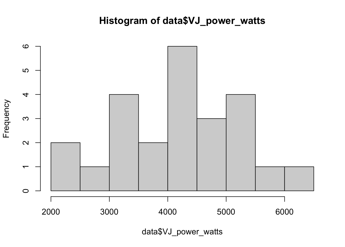
You can make histograms with the hist() function. All you need to do is select the column to plot, which in this case is data$VJ_power_watts, and the rest will be done for you:

hist(x = data$VJ_power_watts)

You could then change the color and labels, create a title, add vertical lines indicating the mean and median (which can each have their own color), change the bins, edit the axes, change the border color, and much more. This is just to give you an idea, in case you’d like to create more complete plots in R.

hist(x = data$VJ_power_watts, 
     col = "lightblue", 
     xlab = "Vertical Jump Power (Watts)",
     main = "Vertical Jump Power",
     border = "black")
abline(v = mean(data$VJ_power_watts), col = "red")
abline(v = median(data$VJ_power_watts), col = "black")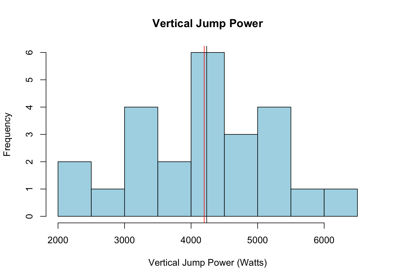

Scatterplot

You can use the plot() function to make scatter plots or various other types of plots. Simply pass your data frame object to the function and R will plot all of the relationships.

plot(x = data)

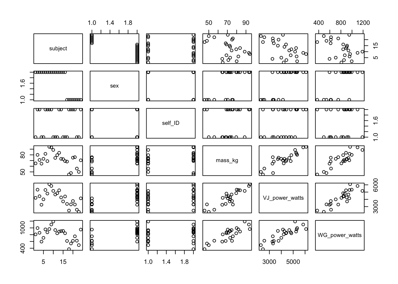
Rather than using all of the data, you can select the relevant variables by subsetting:

plot(data[4:6])

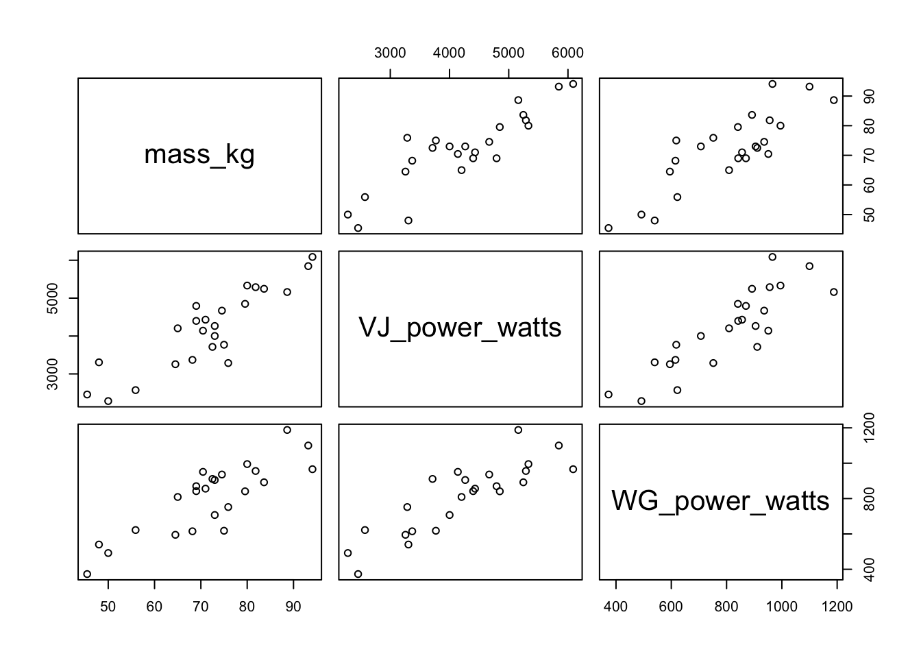
In the code above, the columns 4:6 were selected, which are the columns shown in the plot. You could then color the points by a categorical variable, such as the self_ID variable, which is a variable indicating whether a subject self-identifies as more of a power or endurance athlete. Remember that in order for this to work, the self_ID column needs to be converted to a factor.

plot(data[4:6], col = as.factor(data$self_ID))

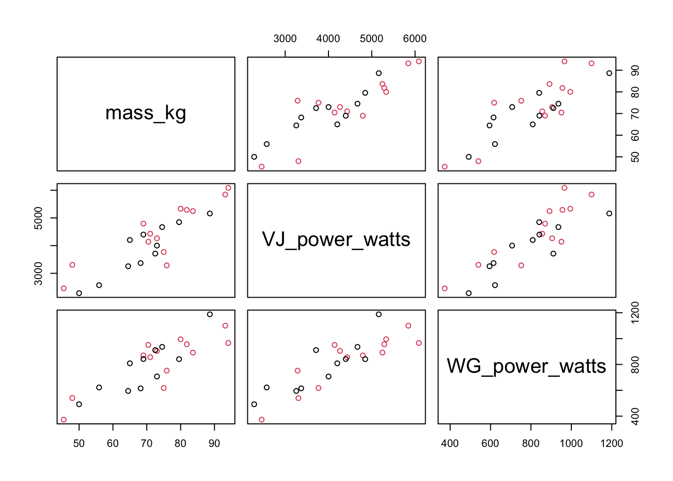
If you wanted to plot the bivariate relationship between two of the variables, you would simply select two of the columns instead of three. Similar to the vertical lines in the histogram plot, you can add the slope and intercept to a plot with the same abline() function. These values were created by performing a linear model and then grabbing the coefficients from the model.

plot(data[4:5])
intercept <- lm(VJ_power_watts ~ mass_kg, data = data)$coeff[1]
slope <- lm(VJ_power_watts ~ mass_kg, data = data)$coeff[2]
abline(coef = c(intercept, slope), col = "red",)

Barplot

You can make bar graphs by using the table() function used earlier in conjunction with the barplot() function.

barplot(table(data$self_ID))

barplot(table(data$self_ID, data$sex))

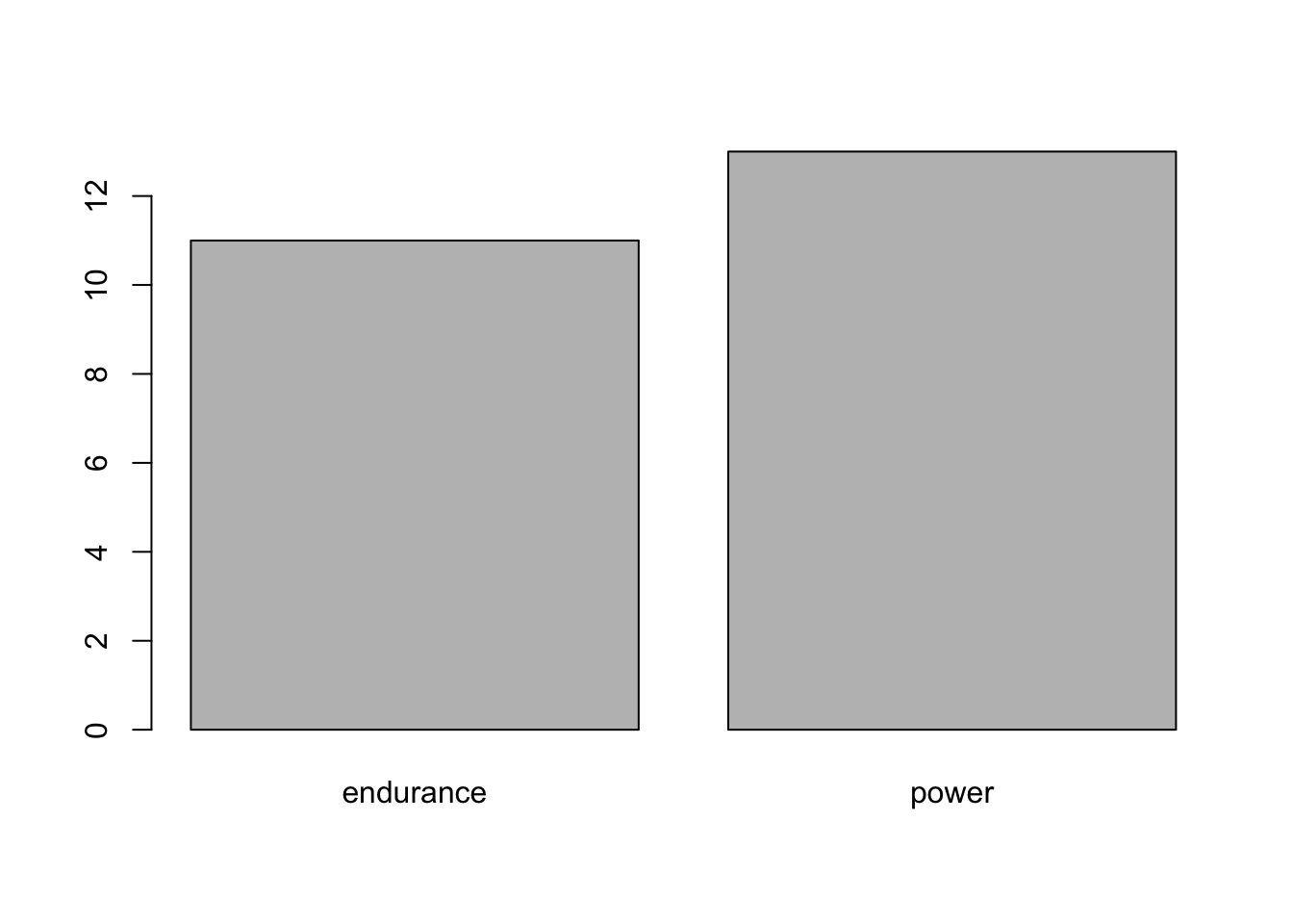
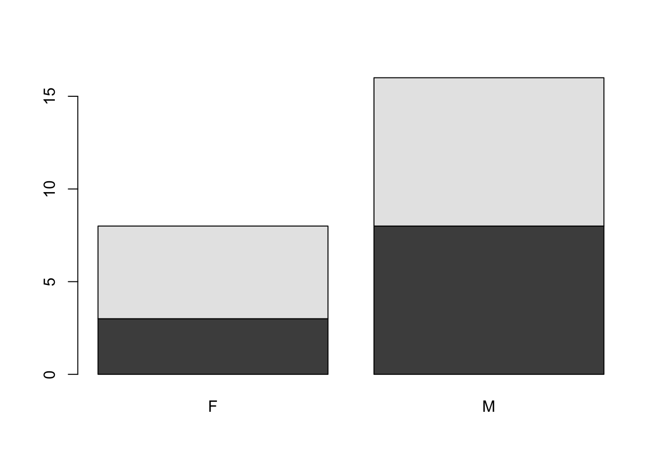
You can have the bars side-by-side instead of stacked by setting beside = TRUE. Notice that you can also generate legends for your plots with the legend() function and then coloring them accordingly.

barplot(table(data$sex, data$self_ID), 
        beside = TRUE, 
        col = c("lightcoral", "lightblue"))
legend("topleft", c("F", "M"), fill = c("lightcoral", "lightblue"))

Boxplot

Boxplots can be created with the boxplots() function. The formatting for this function may seem a little strange. For the formula argument, you’ll first list the y variable followed the x variables. The x variables will be separted by a plus sign. This function automatically converts the sex and self_ID columns to factors for us.

boxplot(formula = VJ_power_watts ~ self_ID + sex, 
        data = data, 
        col = c("lightcoral", "lightgoldenrod", "lightblue", "lightgreen"))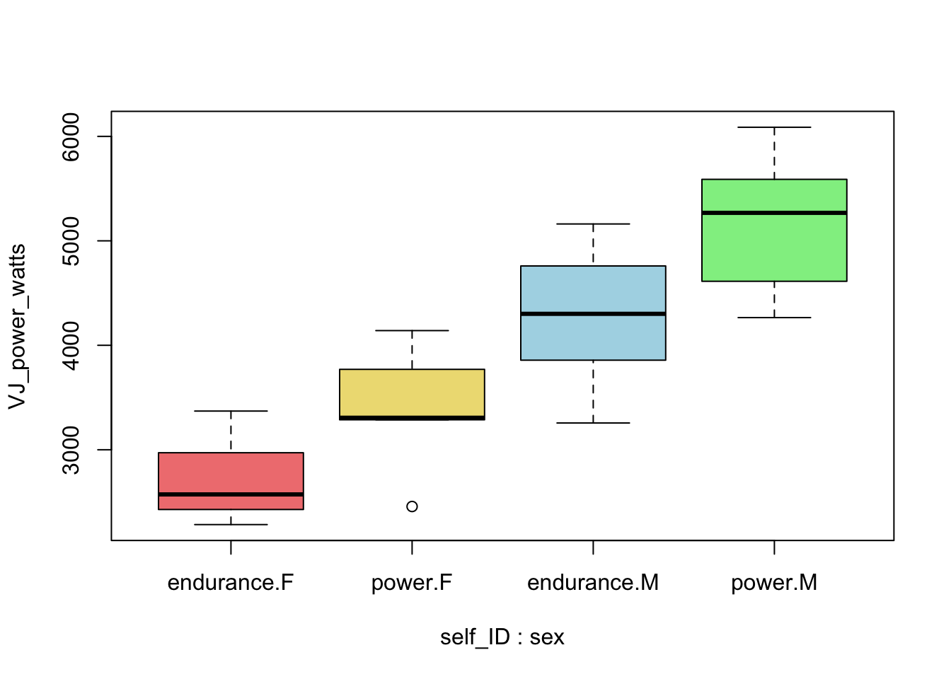

You can view the list of available color options for plots by typing colors() into the console.