13 Analysis of Covariance (ANCOVA)

In this example we’ll use the aov() function for fitting one and two sample t-test models with one continuous predictor, which will take the following form:

\[y_i=\beta_0+\beta_1\left(X1\right)+\beta_2\left(X2\right)+\epsilon_i\]

The code in this chapter only works if you’re following along with the Github folder for this book (which you can download here), you’ve correctly set your working directory to the data folder (which you can learn how to do in Chapter 4, and run the code in the order it appears in this chapter.

Importing

data <- read.csv("power.csv")

Viewing

In this dataset, males and females performed a maximal effort Wingate Test, which is a 30 second test usually performed on a stationary bike that’s used to assess anaerobic leg power. The participant’s maximum achieved power, WG_power_watts, mass, mass_kg, and several other variables were recorded.

head(data)

  subject sex   self_ID  mass_kg VJ_power_watts WG_power_watts
1       1   M endurance 65.00000       4203.498            809
2       2   M     power 80.00000       5332.476            995
3       3   M     power 71.00000       4430.985            856
4       4   M endurance 64.50000       3256.266            595
5       5   M endurance 73.00000       4001.481            707
6       6   M     power 81.81818       5289.559            956

ggplot(data, aes(x = mass_kg, y = WG_power_watts, color = sex)) +
    geom_point() + 
    geom_smooth(method = "lm", se = FALSE) + 
    theme_bw() + 
    scale_color_brewer(palette = "Dark2") +
    labs(title = "Wingate Power vs Mass in Males and Females") + 
    xlab("Mass (kg)") +
    ylab("Wingate Power (Watts)")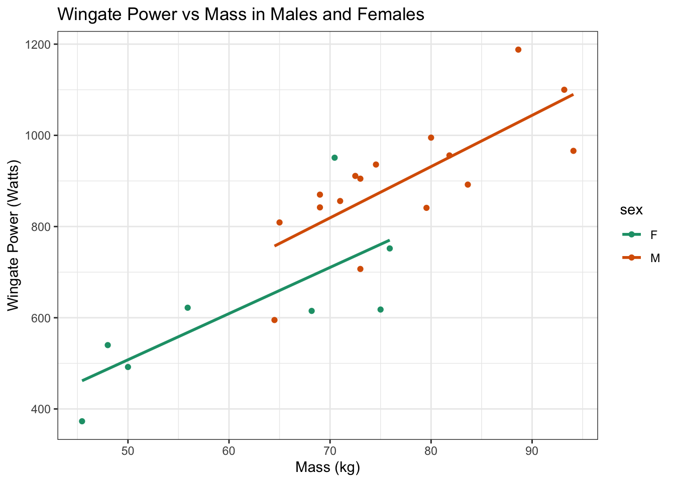

More examples of viewing data can be found in Chapter 5

Modeling

The `aov()`Function

aov(formula, data = NULL, projections = FALSE, qr = TRUE,
    contrasts = NULL, ...)

The aov function has several arguments, but the only ones that need to be specified are the formula and data arguments.

Model

When using the aov() function, the formula argument is set equal to the dependent variable, followed by a tilde, ~, and then the independent variable(s). The data argument is set equal to the object that contains the dataset, which in this example is the object called data.

my_model <- aov(formula = WG_power_watts ~ sex + mass_kg, data = data)

You can use the summary.lm() function to see a summary of the model.

summary.lm(my_model)